lecture12: Normal distribution and simulations

Prashant K

2024-02-22

Recap

In the first 6 weeks we covered

• Basic R

• Tidyverse data manipulations

• Plotting with ggplot

Now we will bring forth these R skills to interact with data to understand the statistics behind t-tests in the next 3 lectures

• Use simulations to generate probability distributions and plot them

Today’s class

The origins of normal distributions and why we see them everywhere

• Central limit theorem visually

• Sample means make normal distributions

• Explore these for yourself with the worksheet (last 30 mins)

Worksheets on the class-worksheets github

Normal distribution

Watch full video/ 3blue1brown (0 - 54 seconds)

How to identify a normal distribution?

• Extremes are less likely than central values (closer to median)
• It is symmetric around the median value
  • Non-symmetric distortions => skew. Ex: Thicker tails on the right => more observations than expected on the right => right-skewed / positively skewed
• We will discuss the technically sound way to identify if data is normally distributed in the next lecture

Galton board and central limit theorem

Central limit theorem in short:

Sum of many random variables makes a normal distribution. Mean involves a sum! (mean <- sum(x) / length(x))

the central limit theorem (CLT) states that, under appropriate conditions, the distribution of a normalized version of the sample mean converges to a standard normal distribution. This holds even if the original variables themselves are not normally distributed. Source: Wikipedia.

Refer textbook for mathematical definition in Introduction to Probability andMathematicalStatistics

Galton board ~ add a random variable (+1 / -1) that determines where the balls end up

Watch full video/ 3blue1brown (1:53 - 5:22)

Why are so many things normally distributed?

Because they could be expressed as a SUM of other hidden variables.

• Heights: We can speculate that height depends on the sum of action of multiple genes, the food/excersise you had everyday till measurement

• Gene expression in a bacterial/cell culture: The sum (or mean) of the expression of the millions of individual cells in the culture makes for an excellent normal distribution!

But it is important to recognize when effects are not strictly additive, such as when feedbacks are involved.

• Income is famously not normally distributed. Due to positive feedback across generations, and that capital gains far outweigh labor gains, there are very few very rich and many many not-very-rich people.

• If your gene has a positive/negative feedback loop (activates/represses itself), then your gene expression will not be normally distributed. You might have a bimodal distribution with 2 peaks!

What is a simulation

Definition from the textbook: Modern stats with R

A key component of modern statistical work is simulation, in which we generate artificial data that can be used both in the analysis of real data (..) and for assessing different (statistical) methods .

Ingredients of a simulation in R

• A random variable

# Pick a random variable (note: rounding is only for the presentation)
rnorm(5, mean = 0, sd = 1) %>% round(2) # Normal random variable (r.v)

[1] -0.23  0.12  0.32  0.14  0.31

sample(letters[1:10], size = 3, replace = TRUE) # sample from a vector

[1] "j" "e" "g"

sample(c(1, -1), size = 1, replace = TRUE) # galton r.v

[1] 1

• Do computations on the random variables

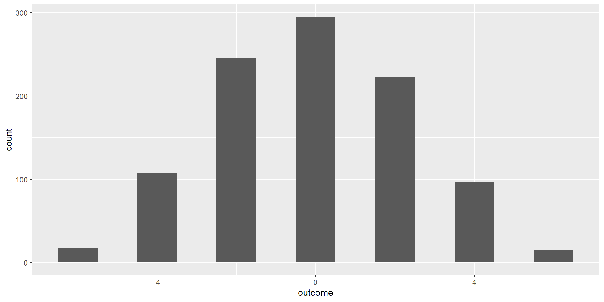
#' calculate sum of `n` random variables
galton_sum <- function(n) {
  galton_series <- sample(c(1, -1), size = n, replace = TRUE)
  sum(galton_series)
}

# each run gives a different outcome
galton_sum(5) ; galton_sum(5); galton_sum(5)

[1] -1

[1] 3

[1] -1

Do the simulation R

• Iterate this many times (avoid for() loops, and use vectorized functions)

galton_simulation <- 
  tibble(
    run_number = 1:10,
    outcome = 
      replicate(n = length(run_number), 
                expr = galton_sum(6))
  ) %>% 
  print()

# A tibble: 10 × 2
   run_number outcome
        <int>   <dbl>
 1          1      -2
 2          2       0
 3          3      -2
 4          4       0
 5          5      -4
 6          6      -2
 7          7      -2
 8          8       6
 9          9      -2
10         10       0

Really do many times

10 is no good, let’s try 1,000?

galton_simulation <- 
  tibble(
    run_number = 1:1e3,
    outcome = 
      replicate(n = length(run_number), 
                expr = galton_sum(6))
  )

Plot results

• Calculate summary statistics and make plots

ggplot(galton_simulation, mapping = aes(outcome)) +
  
  geom_histogram(binwidth = 1, center = 0)

Why are some numbers missing?

Because of the discrete nature of the random variables, odd numbers cannot be made by adding an even number (6) or +1/-1s (if 0 was included, this would be possible)

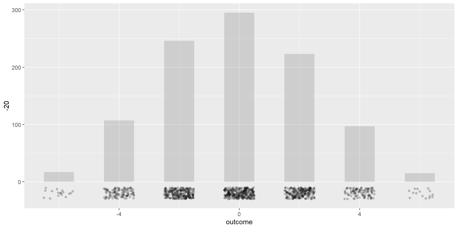
Plot detailed results

Let us plot each outcome on top of the histogram

ggplot(galton_simulation, mapping = aes(x = outcome)) +
  
  geom_histogram(binwidth = 1, center = 0, alpha = 0.2) + 
  geom_jitter(aes(y = -20), 
              position = position_jitter(width = 0.5, height = 10),
              alpha = 0.2)

ggplot(galton_simulation, mapping = aes(x = outcome, y = '?')) +
  
  geom_violin() + 
  # geom_histogram(binwidth = 1, center = 0, alpha = 0.2) + 
  geom_jitter(position = position_jitter(width = 0.5, height = .5),
              alpha = 0.2)

Sampling from a distribution

Collecting a random subset of samples from a larger distribution is another way to begin a simulation. This is the technique behind ~Bootstrapping (will get to it later)

Onto the worksheet now

Please download the qmd worksheet for today from github (scripts/ folder in class-worksheets repository)

Summary

• Understanding normal distributions

• Sum or mean of many random variables produces a normal distribution

• Using R to simulate random events and explore distributions