lecture13
2024-02-27
Recap
Last class covered
How normal distributions are generated: Sum of random variables /
meanof a random sample- Central limit theorem
Used R to simulate random events and explore distributions
Today’s class
Finish segment: How do I test if my data is normal?
q-q plotsandShapiro-WilktestWhat questions do t-tests answer?
t-tests dissected: Layout of a general hypothesis test
Understand sampling distributions, standard error of mean (SEM) and confidence intervals (CI)
Checking for normality
How to check if my data is normally distributed?
- We need metrics that give us the shape of the distribution without having to plot the distribution and staring at it
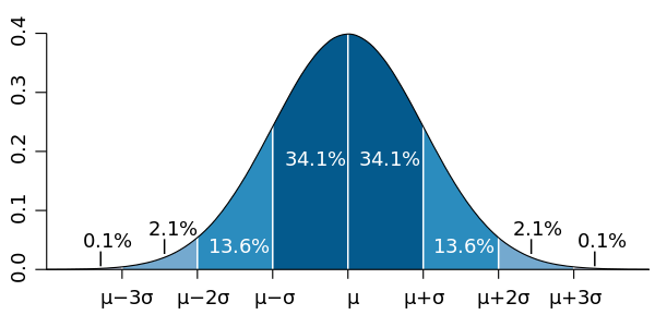
Quantifying the shape of the normal distribution
Median, quartiles
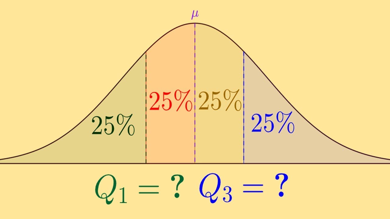
quartiles divide the probability / distribution area into 4 quarters, a more general way is called quantile (note the spelling!)
Quantiles tell us about the distribution shape
Quartiles (4)
Deciles (10)
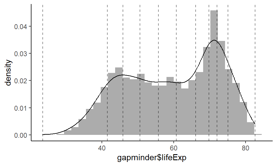
quantiles are cut points dividing the range of a probability distribution into continuous intervals with equal probabilities. Source: Wikipedia
probability distribution = geom_density plot. Hence quantiles divide the range to make equal area under the geom_density curve
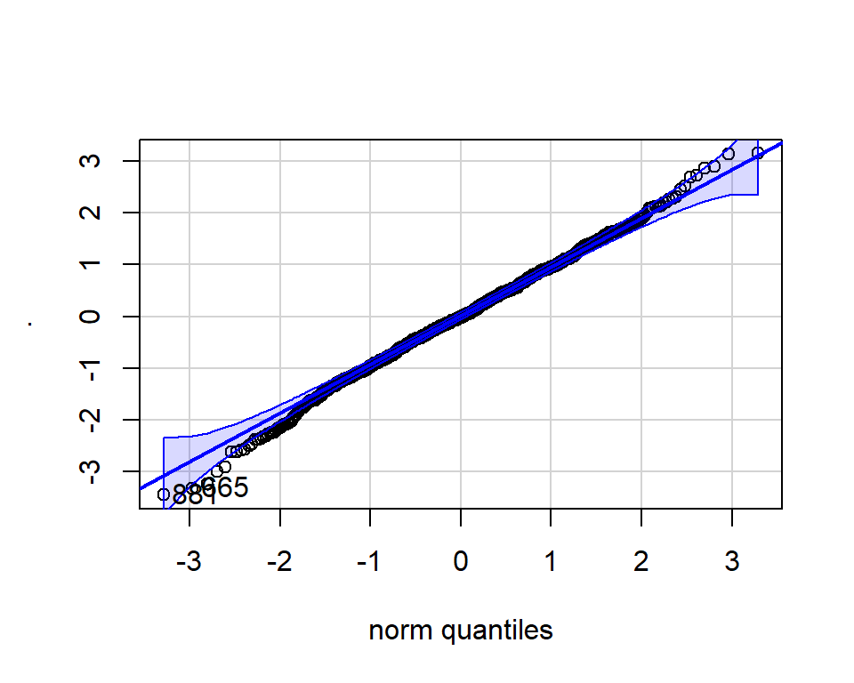
Q-Q plot enables comparison of distribution shapes
If they fall along the line, then it is normal.
Normal distribution
[1] 881 665Non-normal distribution
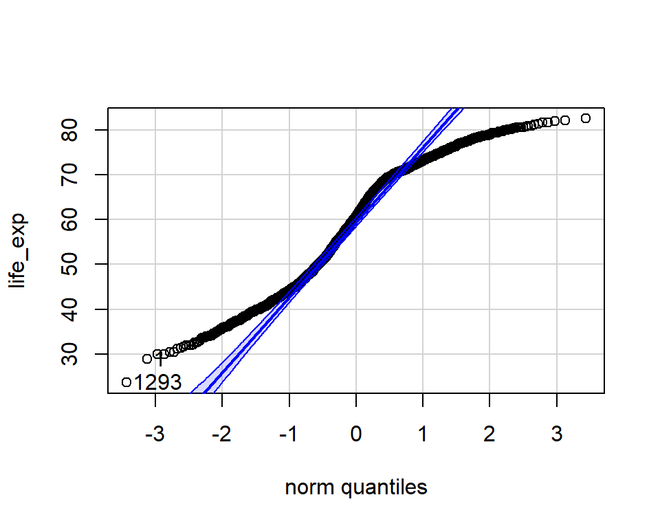
[1] 1293 1Formal Shapiro-Wilk test for normality
What is this testing for?
- NULL hypothesis is that data is normally distributed
- High p-value => Data is normal (hypothesis is accepted)
Normal distribution
    Shapiro-Wilk normality test

data:  .
W = 0.99807, p-value = 0.315
Non-normal distribution
    Shapiro-Wilk normality test

data:  life_exp
W = 0.95248, p-value < 2.2e-16
further reading: statology.org
What are t-tests for?
To make statistical conclusions of this kind based on data
- “Smoking causes cancer”
But causality is really really hard to establish, that is why we talk about correlation/association
“Smoking is associated with cancer”
“Smokers are statistically significantly at a higher risk of having cancer”
“Evidence linking smoking and cancer appeared in the 1920s.” Source: The cigarette controversy, 2007/section: Smoking Causes Cancer: When Did They Know?
What data can test the smoking hypothesis?
2d data
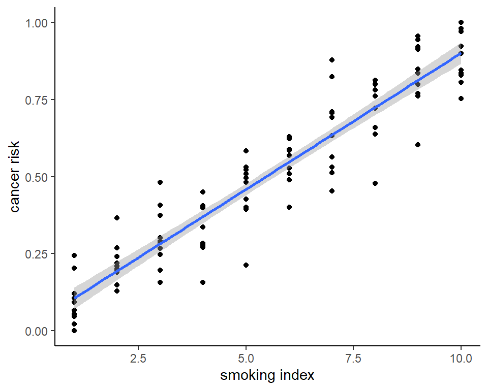
Correlation
Regression (linear/non-linear)
1D data

- t-test
Comparing two numbers vs two samples
Looking at the mean only is not enough:
3.15 is clearly > 2.46, does that alone satisfy the hypothesis?
- We need to account for both the mean and variability, ie) the spread around the mean
This is what the t-statistic encompasses. The t-test tests for a hypothesis based on this statistic
t-tests finds statistical support against a NULL hypothesis
Null hypothesis in english - “smoking is NOT associated with cancer”
In statistical terms - “the samples of smokers and non-smokers came from the same population”
(assumption) For a t-test, this source population is normally distributed
(Other assumption for Student’s t-test) Equal variance between smoker dataset and non-smoker dataset (this can be violated for the
welch t-test)
t-test is calculating difference in means / spread around mean
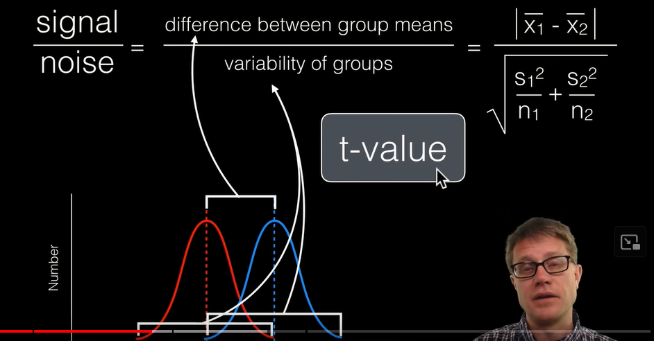
Watch full video here: “Student’s t-test” : Bozeman science/youtube
Sampling distributions
- Sample multiple times from a population (too expensive for a real experiment, so we imagine this)
- Calculate one statistic from the sample (such as
mean) and record it (for each sample) - Plot the statistic across all samples. The statistic is a random variable too dependent on the random sample, hence results in a different value for each sample.
- This results in a distribution (called sampling distribution of
mean/statistic)meanis nice because it follows a normal distribution (due to the central limit theorem!)- it’s mean ~ close approximation to the population mean
- it’s standard deviation = standard error of mean (S.E.M.) ~ \(\sigma\)
- The properties of this distribution are helpful to understand the population which is what we are interested in
Sampling from a population of coloured balls
We will walk through this activity to understand sampling well
- Explanation of sampling with balls in moderndive/chap7
Let us see the sampling distribution
Calculating the sample mean, SEM, CI
Relating this to a 1-sample t-test
References
Great explanation of sample size in 7.2 (FIGURE 7.12) in moderndive/chap7
Summary
q-q plotsandShapiro-Wilktest enable checking data for normalityt-tests answer questions of association such as ‘smoking causes cancer’
t-test = p-value gives the probability that the NULL hypothesis: that both data groups were sampled from the same distribution is
TRUEUnderstood sampling distributions, standard error of mean (SEM) and confidence intervals (CI)
