Understanding (linear) relationships between 2 or more dimensions of data
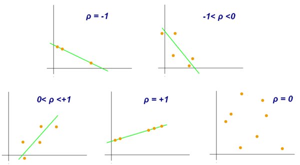
Correlation
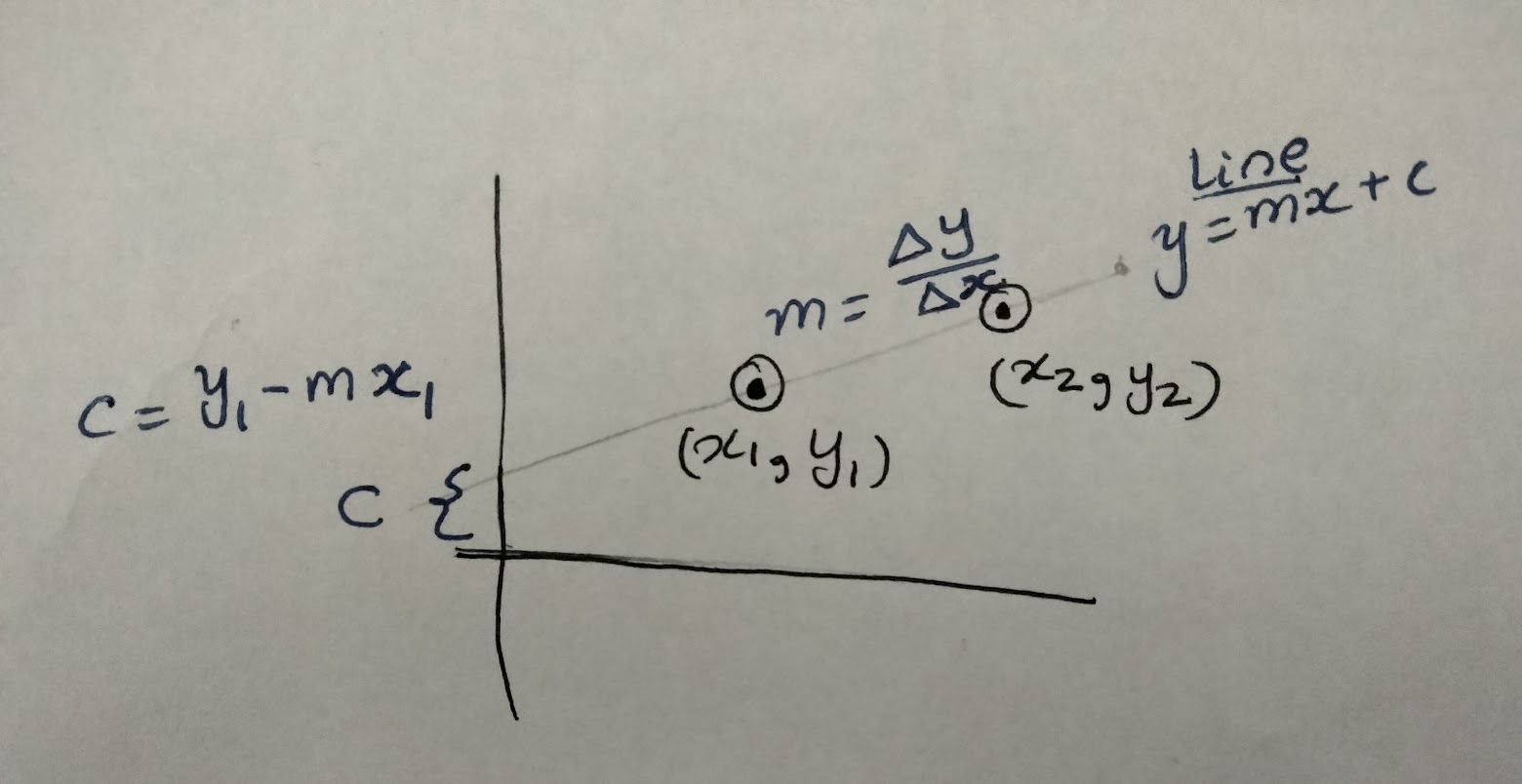
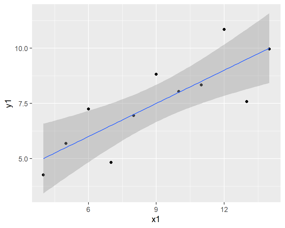
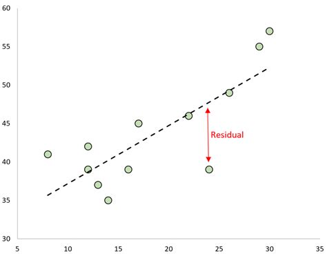
Linear regression
Linear regression is also useful for prediction of y (dependent variable) for new values of x (independent variable)
Using the lm(y ~ x, data = ?) function in R
Interpreting the results : Coefficients, goodness of fit, p-values
Correlation vs linear regression
Correlation coefficient (\(\rho\)) quantifies the linearity of y ~ x (Pearson)
Spearman’s rank correlation coefficient quantifies the monotonicity (y increases when x increases)
Linear regression quantifies the slope of the linearity as well as the degree of fit (\(R^2\))
Many flavours of linear regression
Simple linear regression : \(y = \alpha + \beta x + \eta(0, \sigma)\)