lecture 17: t-test and bootstrapping

Prashant K

2024-03-21

Recap

  • Goal of t-tests: Establish the difference of mean values between 2 samples

  • Reminder on sampling from the red and white balls pictures

  • Reminder on using R to do simulations

  • Today’s class: from sampling distribution -> p-values ; SEM ; CI

Reminder on hypothesis testing

We discussed example in lec13:

Smoking status is statistically significantly associated with higher cancer incidence

NULL hypothesis (for t-test) = Sample means are equal/ samples belong to the same population/distribution

Alternate hypothesis = (choose only 1 per t-test!)

  • Sample means are unequal (two tailed t-test)

  • Sample A’s mean > sample B’s mean (one tailed t-test)

Difference of mean between samples

2 samples = t-test

more samples = ANOVA

Sampling from a population

Population

Sample

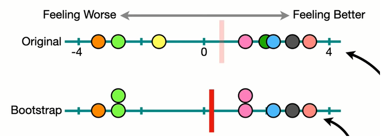
Re-sampling = shuffling within the sample (w replacement)

Sample

Bootstrapped sample (re-sampling, with replacement)

Reminder: Recipe for simulation/lec12

Key difference is how the randomness comes in

  • For simulation, we use rnorm (normal dist, random number) / runif (uniform dist, rv) etc. to generate random numbers from different distributions

  • For sampling, we use sample(population_vector, size = sample_size, replace = FALSE) to select a random sample (subset) of the population

  • For bootstrapping, we use sample(sample_vector, size = sample_size, replace = TRUE) to select a random bootstrap sample from the sample

For repeating steps (iteration), you can use

  • for () loops: beginner friendly

  • map() like vectorized functions: succinct code, needs some head breaking to get used to

Today’s class

  • Doing a t-test in R
  • Using re-sampling distributions to get p-values, Standard Error of Mean (SEM) and confidence intervals (CI)
    • How does this relate to a t-test?
  • Watch the nice Youtube videos linked in the course schedule for lecture 17

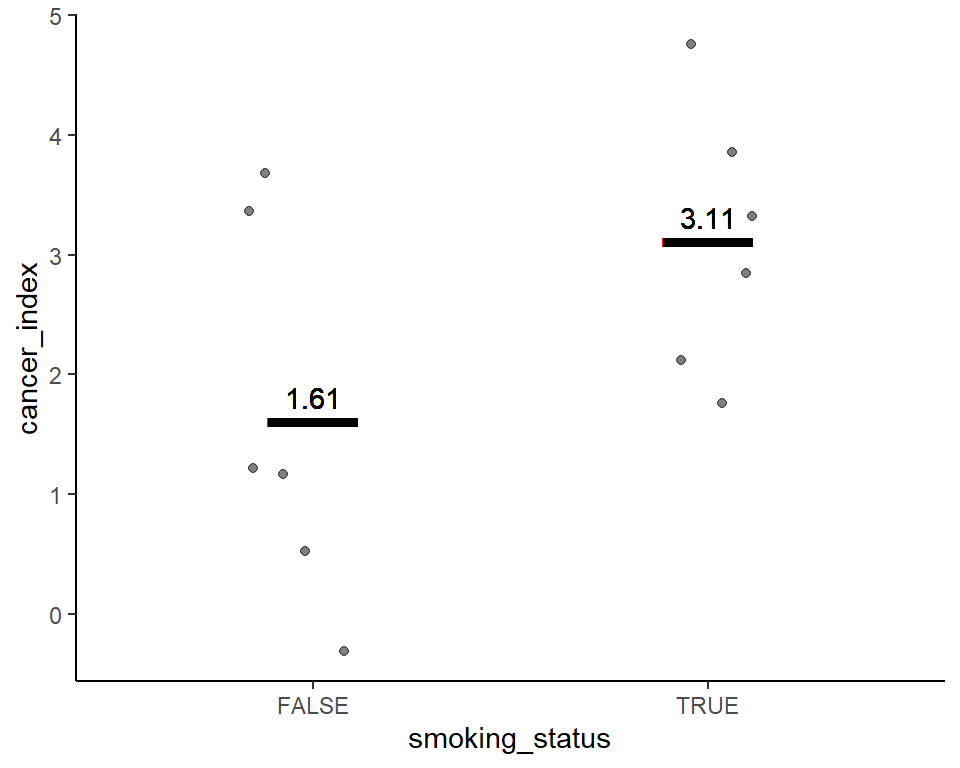
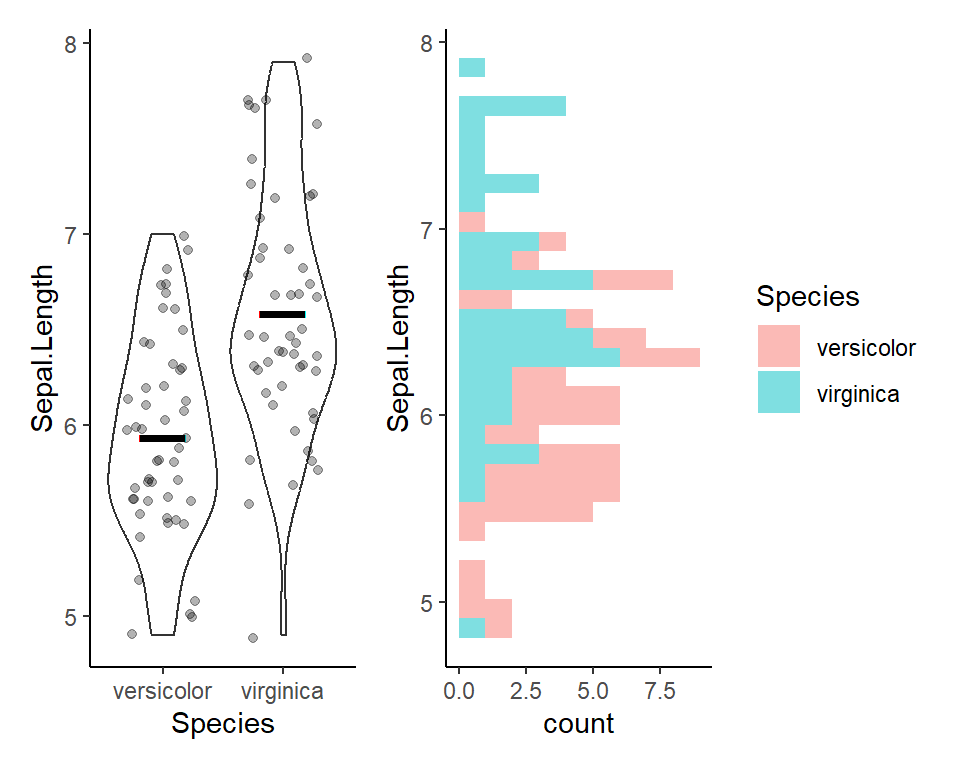
Dataset for t-testing

Many flavours of t-tests

  • 1-sample vs 2-sample

    • >2 samples ~ do ANOVA
  • 1-tailed vs 2-tailed

  • Paired vs unpaired

Visualize before 2-sample t-test

Here’s a plot outlining the data to use for t-test
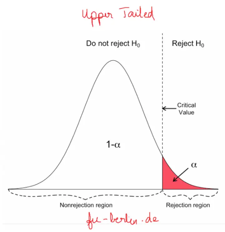
2-sample t-test in R

# Show code and do t-test for vericolor vs virginica
t.test(Sepal.Length ~ Species, data = iris2)

    Welch Two Sample t-test

data:  Sepal.Length by Species
t = -5.6292, df = 94.025, p-value = 1.866e-07
alternative hypothesis: true difference in means between group versicolor and group virginica is not equal to 0
95 percent confidence interval:
 -0.8819731 -0.4220269
sample estimates:
mean in group versicolor  mean in group virginica 
                   5.936                    6.588 

What is p-value?

p-value is the probability that the observed difference of means (or more extreme) can occur by chance if the NULL hypothesis is TRUE

This is calculated by

  • plotting a t-distribution around the null hypothesis mean difference (typically 0)

  • mark the observed mean difference

  • Find the tail of the distribution beyond the observed value

Bootstrapping to understand t-test better

Bootstrapping shows us the variability around the mean, by virtually repeating the experiment a bunch of times

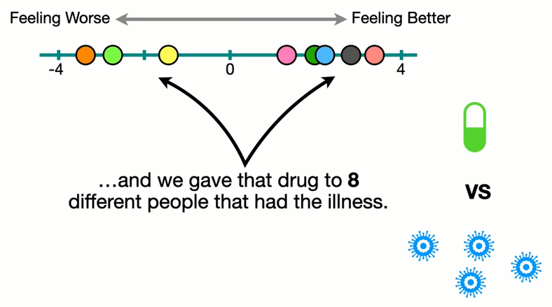
For 1 sample, this is how the bootstrapped distribution looks like

Code
set.seed(1)
sample_1 <- runif(n = 10, -1, 1.5) # make dataset
sample_1 %>% sort() %>% round(2) %>% print # show dataset
 [1] -0.85 -0.50 -0.34 -0.07  0.43  0.57  0.65  1.25  1.27  1.36

1-sample t-test

Null hypothesis (\(H_0\)) ~ [\(\mu = \mu_0\)] => the mean of the data is \(\mu_0\)

  • We will test for: \(\mu = 0\) for this dataset
t_test_1 <- t.test(sample_1, mu = 0) %>% print

    One Sample t-test

data:  sample_1
t = 1.5179, df = 9, p-value = 0.1634
alternative hypothesis: true mean is not equal to 0
95 percent confidence interval:
 -0.1857309  0.9433002
sample estimates:
mean of x 
0.3787847 
t_tst_p <- t_test_1$p.value %>% round(2)
str_c('p-value for t-test is: ', t_tst_p)
[1] "p-value for t-test is: 0.16"

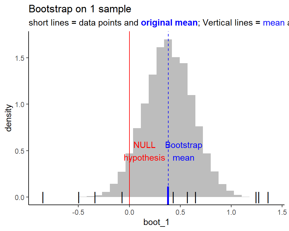
1-sample t-test w bootstrapping

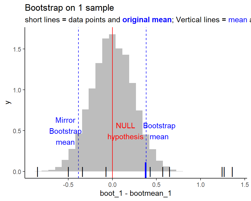
To get p-value from the bootstrapping, we need to find the area of the tails. To facilitate understanding, we shift the distribution to fit the null hypothesis. Which means, the mean of the distribution should be moved to the null hypothesis!
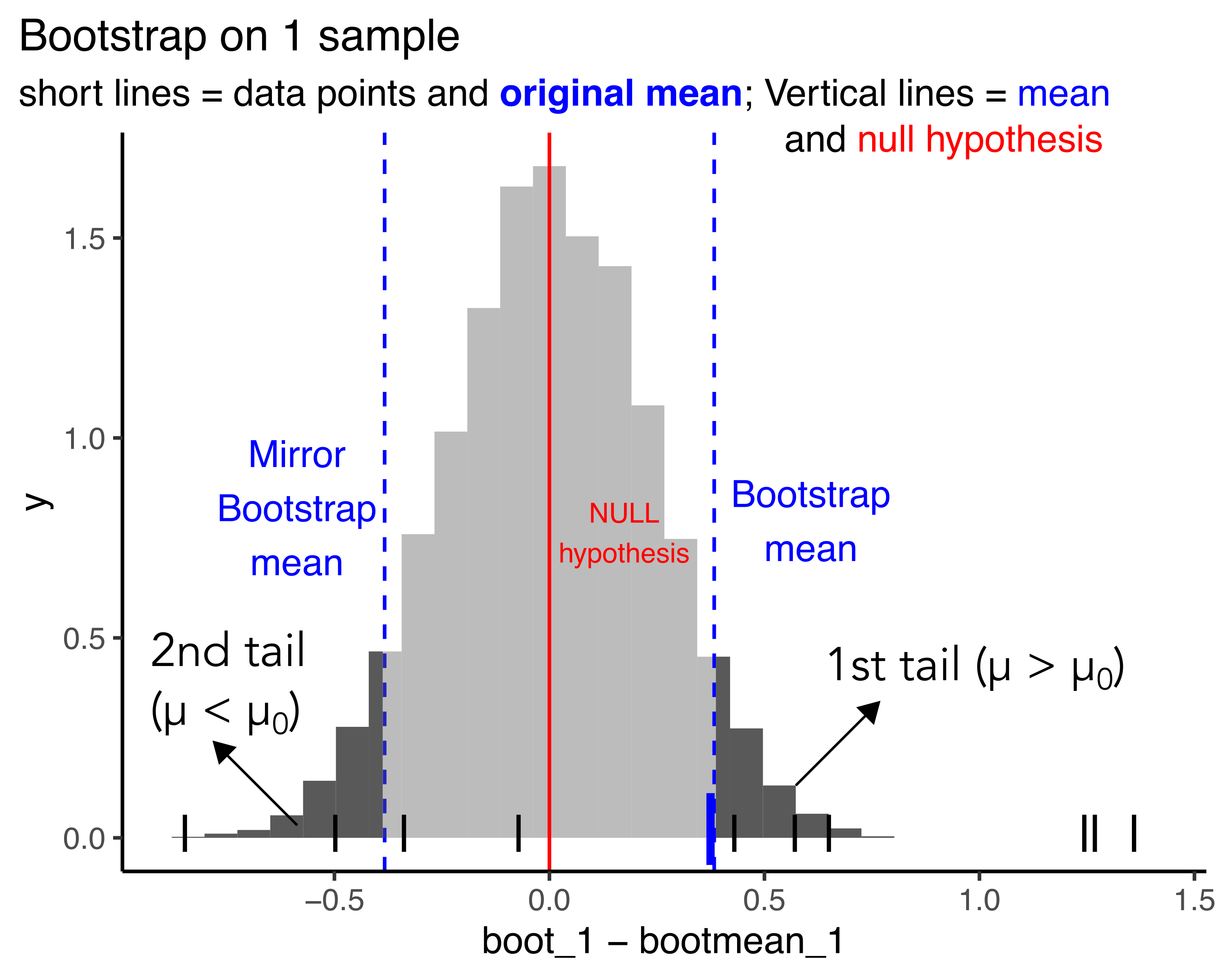
Showing the 2 tails

For a 2 tailed test, the p-value corresponds to the area under these two tails

  • Tail 1: \(\mu > \mu_0\)

  • Tail 2: \(\mu < \mu_0\)

  • Both tails: \(\mu != \mu_0\)

Calculating the p-value from bootstrap dist.

Graphically area is easy to visualize,

For calculation, probability is just the number of values in the tails / total number of values

first_tail <- sum(boot_1 - bootmean_1 > bootmean_1)
second_tail <- sum(boot_1 < 0)  

boot_p_val <- (first_tail + second_tail)/length(boot_1)

str_c('p-value for bootstrapping t-test: ', boot_p_val)
[1] "p-value for bootstrapping t-test: 0.1067"
str_c('p-value for t-test is: ', t_tst_p)
[1] "p-value for t-test is: 0.16"

p-value for t-test is: 0.16

p-value for t-test is: 0.1067

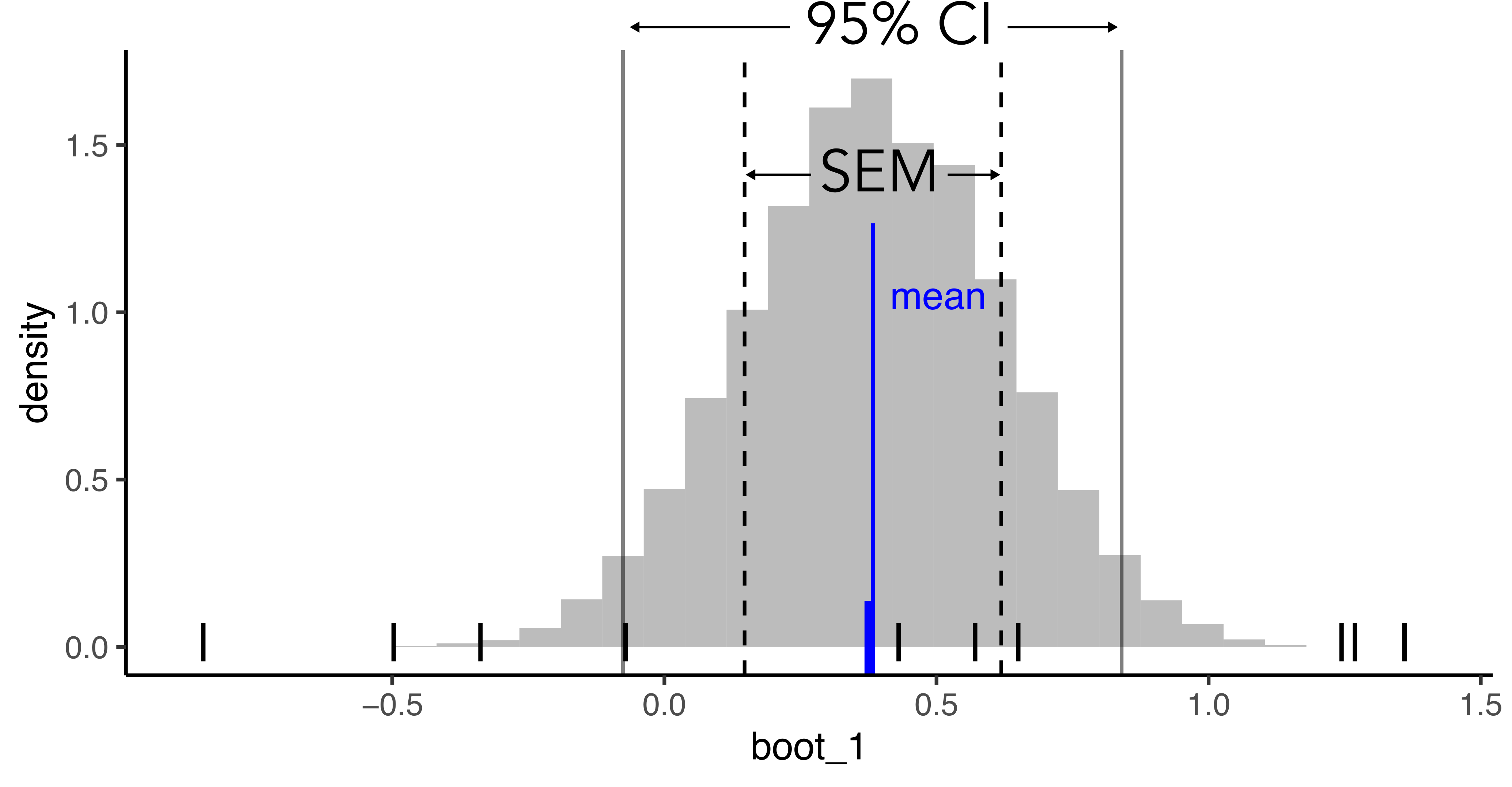
Exploring SEM, CI within bootstrap dist.

  • (SEM) Standard error of mean = std deviation of the bootstrapping distribution

  • (CI) 95% confidence interval => 95% of the mean distribution area lies within this range

Onto the worksheet : 2 samples t-test

Please download/git pull the class17_t-test_bootstrapping.qmd worksheet for today from Github

  • Use the viridis dataset : virginica vs versicolor
    • [second section: Mutate new columns to generate: versicolor (+ 0.5)]
  • Do t.test and record the p-value
  • Do bootstrapping with map
  • Plot histogram, red line with null hypothesis
  • Calculate p value from bootstrap hist
  • Show side by side comparison of both p-values
  • Use automated moderndive:: functions to get the bootstrapped p-value?

Summary

  • Use t.test() to do t-test in R
  • Using bootstraps/re-sampling distributions to get p-values and understand t-test
    • Standard Error of Mean (SEM)
    • Confidence intervals (CI)